Very basic housing project:
Goal:
- Predict the KC county house prices
Importing the necessary libraries
import numpy as np
import pandas as pd
import matplotlib.pyplot as plt
%matplotlib inline

import seaborn as sns
sns.set_style('whitegrid')
import warnings
warnings.filterwarnings('ignore')


from scipy import stats
from sklearn import linear_model
from sklearn import neighbors
from sklearn.metrics import mean_squared_error
from sklearn import preprocessing
from sklearn.model_selection import train_test_split

from math import log
Load data set
data=pd.read_csv('kc_house_data.csv',parse_dates=['date'])
data.describe()
| id | price | bedrooms | bathrooms | sqft_living | sqft_lot | floors | waterfront | view | condition | grade | sqft_above | sqft_basement | yr_built | yr_renovated | zipcode | lat | long | sqft_living15 | sqft_lot15 | |
|---|---|---|---|---|---|---|---|---|---|---|---|---|---|---|---|---|---|---|---|---|
| count | 2.161300e+04 | 2.161300e+04 | 21613.000000 | 21613.000000 | 21613.000000 | 2.161300e+04 | 21613.000000 | 21613.000000 | 21613.000000 | 21613.000000 | 21613.000000 | 21613.000000 | 21613.000000 | 21613.000000 | 21613.000000 | 21613.000000 | 21613.000000 | 21613.000000 | 21613.000000 | 21613.000000 |
| mean | 4.580302e+09 | 5.400881e+05 | 3.370842 | 2.114757 | 2079.899736 | 1.510697e+04 | 1.494309 | 0.007542 | 0.234303 | 3.409430 | 7.656873 | 1788.390691 | 291.509045 | 1971.005136 | 84.402258 | 98077.939805 | 47.560053 | -122.213896 | 1986.552492 | 12768.455652 |
| std | 2.876566e+09 | 3.671272e+05 | 0.930062 | 0.770163 | 918.440897 | 4.142051e+04 | 0.539989 | 0.086517 | 0.766318 | 0.650743 | 1.175459 | 828.090978 | 442.575043 | 29.373411 | 401.679240 | 53.505026 | 0.138564 | 0.140828 | 685.391304 | 27304.179631 |
| min | 1.000102e+06 | 7.500000e+04 | 0.000000 | 0.000000 | 290.000000 | 5.200000e+02 | 1.000000 | 0.000000 | 0.000000 | 1.000000 | 1.000000 | 290.000000 | 0.000000 | 1900.000000 | 0.000000 | 98001.000000 | 47.155900 | -122.519000 | 399.000000 | 651.000000 |
| 25% | 2.123049e+09 | 3.219500e+05 | 3.000000 | 1.750000 | 1427.000000 | 5.040000e+03 | 1.000000 | 0.000000 | 0.000000 | 3.000000 | 7.000000 | 1190.000000 | 0.000000 | 1951.000000 | 0.000000 | 98033.000000 | 47.471000 | -122.328000 | 1490.000000 | 5100.000000 |
| 50% | 3.904930e+09 | 4.500000e+05 | 3.000000 | 2.250000 | 1910.000000 | 7.618000e+03 | 1.500000 | 0.000000 | 0.000000 | 3.000000 | 7.000000 | 1560.000000 | 0.000000 | 1975.000000 | 0.000000 | 98065.000000 | 47.571800 | -122.230000 | 1840.000000 | 7620.000000 |
| 75% | 7.308900e+09 | 6.450000e+05 | 4.000000 | 2.500000 | 2550.000000 | 1.068800e+04 | 2.000000 | 0.000000 | 0.000000 | 4.000000 | 8.000000 | 2210.000000 | 560.000000 | 1997.000000 | 0.000000 | 98118.000000 | 47.678000 | -122.125000 | 2360.000000 | 10083.000000 |
| max | 9.900000e+09 | 7.700000e+06 | 33.000000 | 8.000000 | 13540.000000 | 1.651359e+06 | 3.500000 | 1.000000 | 4.000000 | 5.000000 | 13.000000 | 9410.000000 | 4820.000000 | 2015.000000 | 2015.000000 | 98199.000000 | 47.777600 | -121.315000 | 6210.000000 | 871200.000000 |
Looking for outliers:
data.price.plot(kind='hist',log=True)
<matplotlib.axes._subplots.AxesSubplot at 0x7fb5db910310>
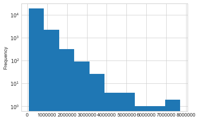
data[data['price']>4e6] # 11 houses greated than 4M
| id | date | price | bedrooms | bathrooms | sqft_living | sqft_lot | floors | waterfront | view | ... | grade | sqft_above | sqft_basement | yr_built | yr_renovated | zipcode | lat | long | sqft_living15 | sqft_lot15 | |
|---|---|---|---|---|---|---|---|---|---|---|---|---|---|---|---|---|---|---|---|---|---|
| 1164 | 1247600105 | 2014-10-20 | 5110800.0 | 5 | 5.25 | 8010 | 45517 | 2.0 | 1 | 4 | ... | 12 | 5990 | 2020 | 1999 | 0 | 98033 | 47.6767 | -122.211 | 3430 | 26788 |
| 1315 | 7558700030 | 2015-04-13 | 5300000.0 | 6 | 6.00 | 7390 | 24829 | 2.0 | 1 | 4 | ... | 12 | 5000 | 2390 | 1991 | 0 | 98040 | 47.5631 | -122.210 | 4320 | 24619 |
| 1448 | 8907500070 | 2015-04-13 | 5350000.0 | 5 | 5.00 | 8000 | 23985 | 2.0 | 0 | 4 | ... | 12 | 6720 | 1280 | 2009 | 0 | 98004 | 47.6232 | -122.220 | 4600 | 21750 |
| 2626 | 7738500731 | 2014-08-15 | 4500000.0 | 5 | 5.50 | 6640 | 40014 | 2.0 | 1 | 4 | ... | 12 | 6350 | 290 | 2004 | 0 | 98155 | 47.7493 | -122.280 | 3030 | 23408 |
| 3914 | 9808700762 | 2014-06-11 | 7062500.0 | 5 | 4.50 | 10040 | 37325 | 2.0 | 1 | 2 | ... | 11 | 7680 | 2360 | 1940 | 2001 | 98004 | 47.6500 | -122.214 | 3930 | 25449 |
| 4411 | 2470100110 | 2014-08-04 | 5570000.0 | 5 | 5.75 | 9200 | 35069 | 2.0 | 0 | 0 | ... | 13 | 6200 | 3000 | 2001 | 0 | 98039 | 47.6289 | -122.233 | 3560 | 24345 |
| 7252 | 6762700020 | 2014-10-13 | 7700000.0 | 6 | 8.00 | 12050 | 27600 | 2.5 | 0 | 3 | ... | 13 | 8570 | 3480 | 1910 | 1987 | 98102 | 47.6298 | -122.323 | 3940 | 8800 |
| 8092 | 1924059029 | 2014-06-17 | 4668000.0 | 5 | 6.75 | 9640 | 13068 | 1.0 | 1 | 4 | ... | 12 | 4820 | 4820 | 1983 | 2009 | 98040 | 47.5570 | -122.210 | 3270 | 10454 |
| 8638 | 3835500195 | 2014-06-18 | 4489000.0 | 4 | 3.00 | 6430 | 27517 | 2.0 | 0 | 0 | ... | 12 | 6430 | 0 | 2001 | 0 | 98004 | 47.6208 | -122.219 | 3720 | 14592 |
| 9254 | 9208900037 | 2014-09-19 | 6885000.0 | 6 | 7.75 | 9890 | 31374 | 2.0 | 0 | 4 | ... | 13 | 8860 | 1030 | 2001 | 0 | 98039 | 47.6305 | -122.240 | 4540 | 42730 |
| 12370 | 6065300370 | 2015-05-06 | 4208000.0 | 5 | 6.00 | 7440 | 21540 | 2.0 | 0 | 0 | ... | 12 | 5550 | 1890 | 2003 | 0 | 98006 | 47.5692 | -122.189 | 4740 | 19329 |
11 rows × 21 columns
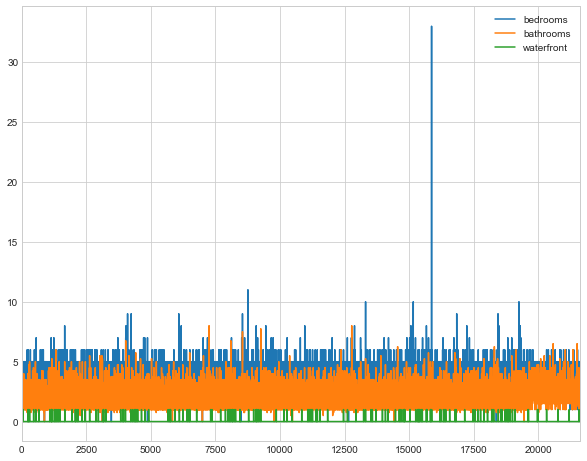
plt.figure(figsize=(10,8))
data.bedrooms.plot(),data.bathrooms.plot(),data.waterfront.plot()
plt.legend()
<matplotlib.legend.Legend at 0x7fb5db4f7110>
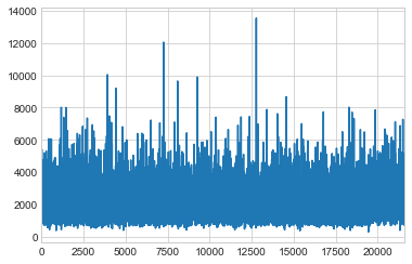
data.sqft_living.plot()
<matplotlib.axes._subplots.AxesSubplot at 0x7fb5db7568d0>
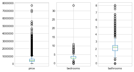
BOX PLOT
fig=plt.figure(figsize=(6,10))

ax1=plt.subplot(331)
ax2=plt.subplot(332)
ax3=plt.subplot(333)
#ax4=plt.subplot(334)
#ax5=plt.subplot(335)
#ax6=plt.subplot(336)
#ax7=plt.subplot(337)


data.boxplot(column='price',ax=ax1)
data.boxplot(column='bedrooms',ax=ax2)
data.boxplot(column='bathrooms',ax=ax3)


plt.suptitle('')
plt.tight_layout()
data[data['bedrooms']>10]
| id | date | price | bedrooms | bathrooms | sqft_living | sqft_lot | floors | waterfront | view | ... | grade | sqft_above | sqft_basement | yr_built | yr_renovated | zipcode | lat | long | sqft_living15 | sqft_lot15 | |
|---|---|---|---|---|---|---|---|---|---|---|---|---|---|---|---|---|---|---|---|---|---|
| 8757 | 1773100755 | 2014-08-21 | 520000.0 | 11 | 3.00 | 3000 | 4960 | 2.0 | 0 | 0 | ... | 7 | 2400 | 600 | 1918 | 1999 | 98106 | 47.5560 | -122.363 | 1420 | 4960 |
| 15870 | 2402100895 | 2014-06-25 | 640000.0 | 33 | 1.75 | 1620 | 6000 | 1.0 | 0 | 0 | ... | 7 | 1040 | 580 | 1947 | 0 | 98103 | 47.6878 | -122.331 | 1330 | 4700 |
2 rows × 21 columns
Removing Outliers
outliers=data.quantile(0.90)
x=data[(data['price']<outliers['price'])]
x=x[(x['bedrooms']< outliers['bedrooms'])]
x=x[(x['bathrooms']< outliers['bathrooms'])]
x=x[(x['sqft_living']< outliers['sqft_living'])]
x.shape
(11712, 21)
data.shape
(21613, 21)
Creating Dummies
x_zipcode=pd.get_dummies(x['zipcode'],drop_first=True)
x=pd.concat([x,x_zipcode],axis=1)
Feature Engineering
x['built_ago']=2017-x['yr_built']
x['have_basement']=np.where(x['sqft_living']>0,1,0)
x['renovated']=np.where(x['yr_renovated']>0,1,0)
x['weighted_bath']=x['bathrooms'] **2
x['weighted_livingspace']=x['sqft_living']**2
x['diff_living']=x['sqft_living']-x['sqft_living15']
x['bed_bath_ratio']=(x['bedrooms']+1)/(x['bathrooms']+1)
y=x.price
x=x.drop(['id','date','zipcode','lat','long','price','yr_built','sqft_basement','bathrooms'],axis=1) # all of them id date zipcode lat long price yr_renovated yr_built sqft_basement bathrooms grade
Train Test Split
# Linear Regression
x_train,x_test,y_train,y_test=train_test_split(x,y,train_size=0.8,random_state=42)
x_train.shape,y_train.shape,x_test.shape,y_test.shape
((9369, 88), (9369,), (2343, 88), (2343,))
Use Linear Regression
reg=linear_model.LinearRegression()
regmodel=reg.fit(x_train,y_train)
y_predtest=reg.predict(x_test)
RMS=mean_squared_error(y_test,y_predtest) ** 0.5
RMS
71972.313409169568
Use Lasso Model:
from sklearn.linear_model import Lasso
ls=Lasso()
l=ls.fit(x_train,y_train)
y_ls_predtest=ls.predict(x_test)
ls_rmse=mean_squared_error(y_test,y_ls_predtest) ** 0.5
ls_rmse
71872.274572752882